If you've been following this series, you've already seen NLP do some impressive things with language.
You've seen how tokenization breaks raw text into individual pieces a program can work with. You've seen POS tagging assign grammatical labels to words. You've seen dependency parsing map the relationships between words in a sentence. And you've seen word sense disambiguation use context to determine whether "bank" refers to a financial institution or the side of a river.
Those techniques are far from academic curiosities. They're useful in their own right and continue to play important roles in many real-world systems. Search engines, information extraction pipelines, document processing systems, and domain-specific NLP applications often rely on linguistic analysis to improve accuracy and relevance.
But there is another challenge we haven't addressed yet.
Many of the algorithms used for search, ranking, classification, clustering, and machine learning operate on numerical representations rather than words and linguistic labels alone. To compare documents mathematically, measure similarity, train models, or rank search results, we need a way to convert text into vectors of numbers.
This process is known as text vectorization.
Bag of Words and TF-IDF are two of the foundational approaches to solving that problem. They don't replace tokenization, POS tagging, dependency parsing, or other linguistic techniques. Instead, they provide a numerical representation that can be used alongside them in larger NLP systems.
These methods are simple enough to understand in an afternoon, powerful enough to have driven production systems for decades, and still widely used today. Modern search engines, retrieval systems, and machine learning pipelines often combine classical techniques such as TF-IDF and BM25 with linguistic analysis and neural models rather than choosing one approach over another.
In this post, we'll explore Bag of Words and TF-IDF from first principles: the intuition behind them, the mathematics that makes them work, and practical Python examples you can run yourself.
The Core Problem: Computers Can't Read Text
Imagine you're building a spam filter. You want your program to look at an email and decide: spam or not spam?
To do that, you need to compare emails somehow. You need to ask questions like: does this email look more like the spam emails I've seen, or more like the legitimate ones?
But you can't compare raw text directly in any meaningful mathematical way. What would it even mean to subtract one sentence from another? How do you calculate the "distance" between "Win a free prize!" and "Your invoice is attached"?
What you need is a way to represent each document as a set of numbers (a vector) so that you can apply all the usual mathematical tools to them: measuring distance, finding similarities, feeding them into classifiers.
This transformation from raw text into numerical vectors is called text vectorization. It's the foundation that everything else in NLP sits on.
One important thing to set expectations correctly before we dive in: the classical methods we're covering today (Bag of Words and TF-IDF) capture shared vocabulary, not meaning. Two documents get similar vectors if they use many of the same words, not simply because they express the same idea. A document about "automobiles" and one about "cars" could look quite different to these methods, even though they cover the same subject. That's one of the limitations we'll come back to, and a big part of why word embeddings and transformers were developed later.
Bag of Words and TF-IDF are the two classic approaches to text vectorization.
Bag of Words: Counting What's There
The Basic Idea
The bag of words model is built on a beautifully simple premise: a document can be represented by the words it contains, and how often they appear.
That's it. You throw away sentence structure, word order, grammar: everything except the raw inventory of words and their counts.
Why "bag"? Because imagine tipping all the words out of a document into a bag and shaking it. The structure is gone. The order is gone. What's left is just a jumbled collection of words. That jumbled collection is your representation.
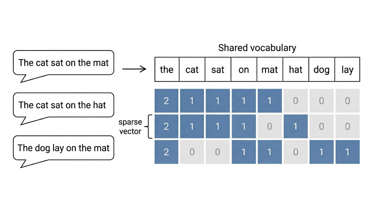
Here's a concrete example. Suppose you have three short documents:
Document 1: "The cat sat on the mat" Document 2: "The cat sat on the hat" Document 3: "The dog lay on the mat"
The first step is to build a vocabulary: the complete list of unique words across all documents.
Vocabulary: [the, cat, sat, on, mat, hat, dog, lay]Now you represent each document as a vector of word counts — one number per word in the vocabulary:
| the | cat | sat | on | mat | hat | dog | lay | |
|---|---|---|---|---|---|---|---|---|
| Document 1 | 2 | 1 | 1 | 1 | 1 | 0 | 0 | 0 |
| Document 2 | 2 | 1 | 1 | 1 | 0 | 1 | 0 | 0 |
| Document 3 | 2 | 0 | 0 | 1 | 1 | 0 | 1 | 1 |
Each row is now a vector of numbers. Documents 1 and 2 share most of the same words, so their vectors look similar. Document 3 shares fewer words with the others, which shows up in the numbers too.
You've just turned text into maths.
Notice something about these vectors: most of the entries are zero. Each document only contains a handful of the words in the full vocabulary, so most positions are empty. This is called a sparse vector, and it's a defining characteristic of both Bag of Words and TF-IDF. In a real corpus with a vocabulary of tens or hundreds of thousands of words, a typical document might use only a few hundred of them, meaning the vast majority of entries in its vector are zero.
This sparsity has practical consequences. Sparse vectors can be stored and computed with efficiently using specialised data structures, but they're very high-dimensional, and all those zeros mean the vectors don't capture much about what words mean, only which words appear. Later in this series we'll look at dense embeddings (compact vectors where every entry carries meaning) which take a fundamentally different approach to representing text. But sparse vectors remain useful and widely deployed, as we'll see.
What Bag of Words Is Actually Good For
Once your documents are vectors, you can do real computation on them. You can measure how similar two documents are by comparing their vectors. You can feed them into a machine learning classifier. You can cluster them, search them, rank them.
The bag of words model works surprisingly well for many tasks:
- Text classification: Is this review positive or negative? The presence of words like "great," "loved," "excellent" versus "terrible," "disappointed," "broken" carries a lot of signal.
- Spam detection: Certain words and phrases appear much more often in spam than in legitimate email.
- Document similarity: Two documents covering the same topic will tend to use many of the same words.
The key insight is that for a lot of real-world tasks, what matters most is which words are present, not the exact order they appear in.
The Obvious Limitations
Bag of words is simple by design, and that simplicity comes with real costs.
Word order is lost entirely. "The dog bit the man" and "The man bit the dog" produce identical bag of words vectors, even though they mean opposite things.
Common words drown out meaningful ones. Words like "the," "a," "is," "and" appear in almost every document. They dominate the word counts but carry almost no useful information. You can partially fix this with a stop word list (a predefined list of common words to ignore) but the underlying problem remains.
Every word is treated as equally important. A document about machine learning that mentions "neural" twice gets the same weight as one that mentions it twenty times. And a rare technical term that appears once gets the same weight as "the" appearing fifty times.
That last problem is exactly what TF-IDF was designed to solve.
TF-IDF: Not All Words Are Created Equal
The Intuition
Think about the word "machine" in a collection of technology articles. It probably appears in a lot of documents. It's somewhat useful for identifying tech content, but it's not very distinctive.
Now think about the word "backpropagation." If that word appears in a document, you know a lot about what that document is about. It's rare in most text, but highly specific and meaningful in context.
The core intuition behind TF-IDF is: a word is important if it appears a lot in this specific document, but not in many other documents.
Words that appear everywhere are not very useful for distinguishing one document from another. Words that appear in only a few documents are highly distinctive. A good word representation should reward distinctive words and discount common ones.
TF-IDF (Term Frequency–Inverse Document Frequency) formalises this intuition with a simple formula.
Term Frequency
Term frequency measures how often a word appears in a document.
The simplest version is a raw count: if "neural" appears 4 times in a document, its term frequency is 4. In practice, implementations vary — some use the raw count, some normalise by dividing by the total number of words in the document (so longer documents don't automatically produce higher scores), and some apply logarithmic scaling to reduce the impact of words that appear very many times. Scikit-learn's `TfidfVectorizer`, for instance, uses a specific variant under the hood. The core idea is the same across all of them: measure how prominent this word is within this document.
The normalised version looks like this:
TF(word, document) = (number of times word appears in document) / (total words in document)For example, if "neural" appears 4 times in a 200-word document:
TF = 4 / 200 = 0.02This measures local importance: how much does this word dominate this particular document?
Inverse Document Frequency
Inverse document frequency measures how rare or common a word is across the entire collection.
IDF(word) = log( total number of documents / number of documents containing word )If a word appears in every document, the fraction inside the log becomes 1, and log(1) = 0. The IDF is zero. That word gets no weight at all.
If a word appears in only 1 out of 1,000 documents, the fraction is 1,000, and log(1,000) is a large number. That word gets a high IDF score: it's highly distinctive.
The logarithm is there to compress the scale. Without it, a word appearing in 1 out of 1,000,000 documents would get a weight a thousand times higher than a word appearing in 1 out of 1,000. The log smooths that out.
Putting Them Together
The TF-IDF score for a word in a document is simply:
TF-IDF(word, document) = TF(word, document) × IDF(word)Words that are frequent in this document and rare across the collection get high scores. Words that are common everywhere get scores near zero.
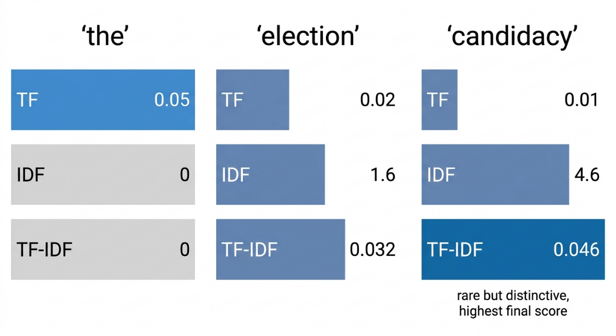
Let's work through a simple example. Suppose you have a collection of 1,000 news articles.
| Word | TF in article | Documents containing word | IDF | TF-IDF |
|---|---|---|---|---|
| "the" | 0.05 | 1,000 (all of them) | log(1) = 0 | 0.000 |
| "election" | 0.02 | 200 articles | log(5) ≈ 1.6 | 0.032 |
| "candidacy" | 0.01 | 10 articles | log(100) ≈ 4.6 | 0.046 |
Even though "the" has the highest term frequency, it gets a TF-IDF of zero because it appears in every document. "Candidacy" is rarer and more distinctive, so it gets the highest score despite appearing less often in this specific article.
This is exactly what you'd want. If you're trying to understand what makes this article distinct, "the" tells you nothing. "Candidacy" tells you a lot.
The TF-IDF Vectorizer: From Concept to Tool
In practice, you rarely compute TF-IDF by hand. You use a TF-IDF vectorizer: a ready-made tool that takes a collection of documents and transforms each one into a TF-IDF vector automatically.
The vectorizer handles all the bookkeeping: building the vocabulary, computing term frequencies, calculating IDF scores across the entire corpus, and assembling the final document-term matrix.
The output is the same shape as a bag of words matrix (rows are documents, columns are words) but now each cell contains a TF-IDF score instead of a raw count.
TF-IDF in Python
Python's scikit-learn library includes a `TfidfVectorizer` that makes this trivially easy.
from sklearn.feature_extraction.text import TfidfVectorizer

# Your documents
documents = [
    "The cat sat on the mat",
    "The cat sat on the hat",
    "The dog lay on the mat"
]

# Create and fit the vectorizer
vectorizer = TfidfVectorizer()
tfidf_matrix = vectorizer.fit_transform(documents)

# See the vocabulary
print(vectorizer.get_feature_names_out())
# ['cat', 'dog', 'hat', 'lay', 'mat', 'on', 'sat', 'the']

# See the TF-IDF scores for document 1
print(tfidf_matrix[0].toarray())
The `fit_transform` call does everything at once: it learns the vocabulary and IDF weights from your documents (`fit`), then transforms each document into a TF-IDF vector (`transform`).
If you later want to transform new documents using the same vocabulary and IDF weights (which you almost always do when building a real system) you call `transform` alone:
new_docs = ["The cat lay on the hat"]
new_vectors = vectorizer.transform(new_docs)
You can also use `CountVectorizer` if you just want raw word counts (the bag of words approach):
from sklearn.feature_extraction.text import CountVectorizer

bow_vectorizer = CountVectorizer()
bow_matrix = bow_vectorizer.fit_transform(documents)
Both vectorizers support useful parameters for cleaning your text automatically:
vectorizer = TfidfVectorizer(
    stop_words='english',       # Remove common English stop words
    max_features=10000,         # Only keep the 10,000 most frequent words
    ngram_range=(1, 2),         # Include both single words and two-word phrases
    min_df=2                    # Ignore words that appear in fewer than 2 documents
)
A Practical Example: Finding Similar Documents
Here's a slightly more realistic use case: using TF-IDF vectors to find which documents are most similar to a query.
from sklearn.feature_extraction.text import TfidfVectorizer
from sklearn.metrics.pairwise import cosine_similarity
import numpy as np

# A small collection of descriptions
documents = [
    "Machine learning algorithms learn patterns from data",
    "Deep learning uses neural networks with many layers",
    "Natural language processing handles text and speech",
    "Computer vision processes images and video",
    "Neural networks are inspired by the human brain"
]

# Fit and transform
vectorizer = TfidfVectorizer()
tfidf_matrix = vectorizer.fit_transform(documents)

# A search query
query = ["neural networks and deep learning"]
query_vector = vectorizer.transform(query)

# Calculate similarity between query and all documents
similarities = cosine_similarity(query_vector, tfidf_matrix).flatten()

# Rank documents by similarity
ranked = np.argsort(similarities)[::-1]
print("Most similar documents:")
for i in ranked:
    print(f"  {similarities[i]:.3f} — {documents[i]}")
Output:
Most similar documents:
  0.712 — Neural networks are inspired by the human brain
  0.634 — Deep learning uses neural networks with many layers
  0.000 — Machine learning algorithms learn patterns from data
  0.000 — Natural language processing handles text and speech
  0.000 — Computer vision processes images and video
The query "neural networks and deep learning" correctly identifies the two most relevant documents. Documents that don't mention neural networks at all score zero.
Notice what TF-IDF is actually doing here: it's matching shared terms, not understanding concepts. It found the right documents because the query and those documents happen to use the same words. If one of our documents had said "artificial neurons arranged in layers" instead of "neural networks," TF-IDF would have given it a score of zero. The terminology doesn't overlap, so the vectors don't either. This is the core limitation of all sparse, vocabulary-based approaches. It works well when related documents use consistent terminology, which is true in many real-world settings. When it breaks down, that's where dense embeddings and semantic search come in.
This term-matching approach is essentially how document search worked for decades — and in many systems, it still does.
Bag of Words vs TF-IDF: When to Use Which
Both approaches transform text into vectors. The difference is what those numbers mean and how much signal they carry.
Use Bag of Words (raw counts) when: - Your task is simple and you want maximum interpretability - You're working with very short texts where document length doesn't vary much - You're doing a quick baseline before trying something more sophisticated
Use TF-IDF when: - Your documents vary in length (longer documents shouldn't automatically dominate) - You want distinctive terms to be weighted more heavily than ubiquitous ones - You're doing search, document similarity, or text classification where specificity matters
In practice, TF-IDF almost always outperforms raw bag of words for text classification and search tasks. It's the default choice when you want a classical vectorization approach.
Where These Methods Fit in Modern NLP
If TF-IDF has been around since the 1970s, you might wonder whether it's still worth learning.
The honest answer: yes, absolutely. And not just for historical context.
Transformer models like BERT and GPT brought contextual embeddings to NLP, which capture meaning, sentence structure, and semantic relationships in ways sparse methods can't. That was a genuine step forward for many tasks. But it didn't make sparse retrieval disappear. The story is more nuanced than "new methods replaced old ones."
In practice, many production systems today use hybrid architectures: they run a sparse retrieval step (BM25, TF-IDF) alongside a dense neural retrieval step, then combine the results. Each component handles what it's good at. Sparse methods are fast, interpretable, and excellent at exact keyword matching. Dense methods are better at semantic similarity: finding documents that mean the same thing even when they use different words. Neither has made the other obsolete. Classical NLP techniques — tokenization, lemmatization, POS tagging, dependency parsing, TF-IDF, and the retrieval pipelines built around them — remain important parts of real production systems.
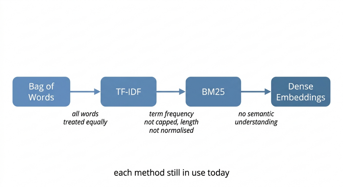
TF-IDF's direct successor, BM25, is one of the most widely deployed ranking algorithms in the world right now. BM25 takes the core TF-IDF idea and fixes two specific weaknesses: it handles diminishing returns on term frequency (the 50th mention of a word shouldn't count as much as the 5th), and it normalises more gracefully for document length. Elasticsearch, OpenSearch, and most modern search engines use BM25 as their default relevance model. It's also the sparse retrieval component in many of those hybrid systems mentioned above. We'll cover BM25 in the next post. Once you've understood TF-IDF, it clicks almost immediately.
Understanding Bag of Words and TF-IDF gives you the conceptual foundation to understand why every subsequent approach works differently, and what specific problem each one was built to solve. Dense embeddings exist because sparse methods can't capture meaning across different vocabulary. BM25 exists because raw TF-IDF has specific edge cases in term weighting and length normalisation. Each step in the progression was motivated by a concrete limitation of what came before — not a wholesale replacement of it.
Every serious NLP practitioner knows these methods. They're the starting point for a reason.
What Comes Next
We've now covered how text gets turned into numbers — the prerequisite for almost every NLP task that follows.
The immediate next step is BM25: the direct evolution of TF-IDF that fixes its two most significant weaknesses and has become the default ranking algorithm inside most modern search engines. If you search anything on Elasticsearch or use a hybrid retrieval system, BM25 is almost certainly involved. Because it builds directly on what you've just learned, it's the natural next post.
After that, we'll go deeper into what you can do with these vectors — the machine learning models that sit on top of text vectorization, and the neural architectures that eventually pushed beyond classical methods altogether. That includes word embeddings like Word2Vec and GloVe, which represent words as dense vectors rather than sparse counts, and eventually the contextual embeddings that power modern AI.
Learn This at Fondra Labs
This post is part of our NLP Foundations series, where we build up practical AI knowledge one concept at a time, from text processing basics all the way to the systems powering modern AI.
At Fondra Labs, we teach AI from production reality, not hype. Every topic in this series is here because it genuinely matters when you sit down to build something real.
If this was useful, explore the rest of the blog. We cover machine learning, deep learning, NLP, and the practical skills that turn understanding into building.
Frequently Asked Questions
Javier Aguirre
Teaching AI from production reality, not hype.
Build your AI Foundations
Get the free checklist that production engineers use to avoid these common RAG pitfalls.
Get the Free Guide