If you've landed here fresh from a search engine, welcome. This post is about one of the most important ideas in modern AI: how computers represent the meaning of words as numbers.
If you've been following this series, you'll know we recently covered BM25: a keyword-based search algorithm that scores documents by matching the exact words in a query against the exact words in a document. If you haven't read that one yet, no problem, here's the short version: BM25 is excellent at finding documents that share vocabulary with your query, and it powers the search behind tools like Elasticsearch. But it has a hard ceiling. It matches words, not meaning.
That ceiling is the problem this post solves.
If you search for "car repair" using BM25, it will not find a document about "automobile maintenance" unless those exact words appear. The two phrases mean the same thing, but BM25 doesn't know that. It just sees two different strings of characters. Same with "heart attack" and "myocardial infarction." Same with "cheap" and "affordable." Keyword search is fast and reliable, but it has no idea what words actually mean.
Word embeddings were created to fix exactly this. Instead of treating every word as an isolated label, embeddings give each word a position in a kind of map, where words with similar meanings are placed close together and words with different meanings are placed far apart. "Car" and "automobile" end up as neighbours on that map. "King" and "queen" end up as neighbours. The meaning of a word gets captured by where it sits, and that position can be compared and measured.
This is the idea that connects classical NLP to modern deep learning. Once you understand word embeddings, everything else in modern NLP, including transformers, BERT, and large language models, becomes much easier to follow.
The Core Idea: Words as Points in Space
Before getting into specific methods, let's build the intuition.
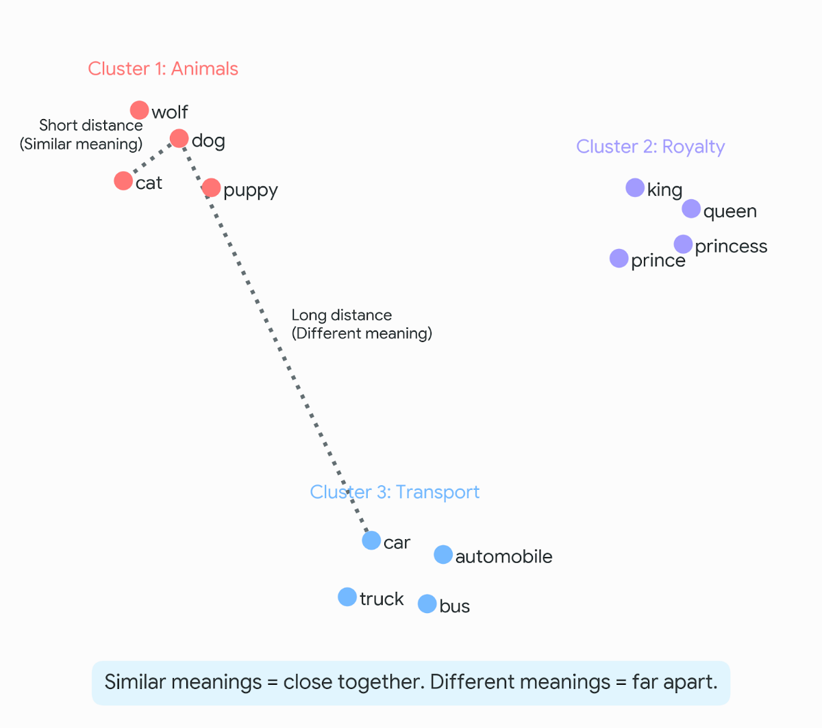
Imagine a map. Every word in the English language gets placed somewhere on that map. Words with similar meanings are placed near each other. Words with different meanings are placed far apart.
Now imagine that map has not two dimensions like a piece of paper, but 300. Or 768. Or 1536. That's hard to picture (nobody can picture 300 dimensions), but the principle is the same: each word gets a location, and that location captures something about its meaning.
That location is represented as a list of numbers. A word like "cat" might be represented as something like `[0.2, -0.5, 0.8, 0.1, ...]` with hundreds of numbers in the list. Each number is one coordinate in that high-dimensional space. The numbers themselves don't have obvious meanings, but together they encode where the word sits relative to all other words.
This list of numbers is called a word vector or a word embedding. The two terms mean the same thing.
Here's what makes this useful. In this space:
- "Dog" and "cat" are close (both domestic animals)
- "Dog" and "wolf" are close (biologically related)
- "Dog" and "aeroplane" are far apart
- "King" minus "man" plus "woman" lands very close to "queen"
That last one is worth pausing on. It means the map has captured something real about the relationship between royalty and gender. You can literally do arithmetic on words and get sensible answers. King is to man what queen is to woman, and the numbers reflect that.
That relationship wasn't hand-programmed. It emerged from training a model on billions of sentences and letting it figure out which words tend to appear in similar contexts. More on how that works in the next section.
Word2Vec: Learning Meaning from Context
Word2Vec is the model that made word embeddings practical and popular. Published by a team at Google in 2013, it showed that you could train high-quality word vectors efficiently on large amounts of text, and that those vectors genuinely captured the meaning and relationships between words.
The key idea behind Word2Vec comes from a simple observation about language:
"You shall know a word by the company it keeps." J.R. Firth, 1957
In plain terms: words that appear in similar contexts tend to have similar meanings. Think about it. "Dog" and "cat" both follow the word "my" regularly. Both appear near words like "pet," "vet," "food," "walk." They both precede "is hungry." Because they keep similar company, they end up with similar vectors.
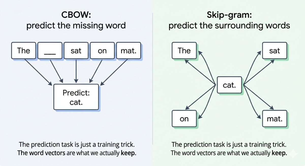
Word2Vec learns these vectors by training a small neural network on a fill-in-the-blank style task. There are two versions of the task:
CBOW (Continuous Bag of Words): given the words around a blank, predict what goes in the blank. Given ["The", "\\\_", "sat", "on", "the", "mat"], predict "cat".
Skip-gram: given one word, predict the words around it. Given "cat", predict ["The", "sat", "on", "the", "mat"].
The fill-in-the-blank task is not the actual goal. It's a training trick. By forcing the neural network to get good at this task, we force it to build up internal representations of each word that capture its meaning. Those internal representations, one per word, are the word vectors we actually care about.
The result: words that are used in similar contexts end up with similar vectors. You can add and subtract these vectors and get sensible answers. The famous example:
vector("king") - vector("man") + vector("woman") ≈ vector("queen")
Think of it this way. The vector from "man" to "king" captures the concept of royalty. Adding that same concept to "woman" brings you to "queen." This arithmetic works because the training process has learned to place words in a consistent, structured way.
Word2Vec in Practice
Word2Vec is available through the `gensim` library in Python:
from gensim.models import Word2Vec

# Your corpus: a list of tokenized sentences
sentences = [
    ["the", "cat", "sat", "on", "the", "mat"],
    ["the", "dog", "ran", "through", "the", "park"],
    ["cats", "and", "dogs", "are", "common", "pets"],
    ["the", "cat", "chased", "the", "dog"],
    ["dogs", "love", "to", "run", "in", "the", "park"]
]

# Train Word2Vec
model = Word2Vec(sentences, vector_size=50, window=3, min_count=1, epochs=100)

# Get the vector for a word
cat_vector = model.wv["cat"]
print("Vector for 'cat':", cat_vector[:5], "...")  # First 5 dimensions

# Find similar words
similar = model.wv.most_similar("cat", topn=3)
print("Most similar to 'cat':", similar)
Output (will vary slightly due to random initialisation):
Vector for 'cat': [ 0.023 -0.041  0.089  0.012 -0.067] ...
Most similar to 'cat': [('dog', 0.94), ('cats', 0.91), ('dogs', 0.87)]
Even with this tiny five-sentence corpus, the model has learned that "cat" and "dog" are related. With a real corpus of millions of sentences, the vectors become much richer and more accurate.
In practice, most people don't train Word2Vec from scratch. They download pretrained vectors that someone else already trained on massive amounts of text (Google News, Wikipedia, or Common Crawl) and use them directly. The Google News vectors were trained on 100 billion words. There's no need to redo that work.
GloVe: A Different Approach to the Same Goal
GloVe (Global Vectors for Word Representation) was published by researchers at Stanford in 2014. It produces similar results to Word2Vec but gets there differently.
Where Word2Vec learns by predicting nearby words one context window at a time, GloVe takes a step back and looks at the whole corpus at once. It counts how often every word appears near every other word across all the text, builds a giant table of those counts, and then finds vectors that mathematically match those counts as closely as possible.
The end result is similar: words with related meanings end up with similar vectors, and you can still do word arithmetic. The practical difference between GloVe and Word2Vec is small and depends on the task. For most applications, pretrained vectors from either model work well.
GloVe vectors are available pre-trained on several large datasets (Wikipedia, Twitter, Common Crawl) and can be loaded directly:
import numpy as np

# Load pretrained GloVe vectors (download from https://nlp.stanford.edu/projects/glove/)
# This example uses the 50-dimensional vectors trained on Wikipedia

def load_glove_vectors(filepath):
    embeddings = {}
    with open(filepath, 'r', encoding='utf-8') as f:
        for line in f:
            values = line.split()
            word = values[0]
            vector = np.array(values[1:], dtype='float32')
            embeddings[word] = vector
    return embeddings

# glove = load_glove_vectors('glove.6B.50d.txt')

# Once loaded:
# cat_vector = glove['cat']
# dog_vector = glove['dog']
# similarity = np.dot(cat_vector, dog_vector) / (np.linalg.norm(cat_vector) * np.linalg.norm(dog_vector))
Both Word2Vec and GloVe are what we call static embeddings: every word gets exactly one fixed vector, no matter where it appears. The word "bank" always gets the same vector, whether it's in a sentence about money or a sentence about a riverbank. This is a significant limitation, and it leads us to the next generation of models.
The Problem with Static Embeddings
Static embeddings have one fixed vector per word, decided during training and never changed.
This creates a real problem with words that have multiple meanings. The word "bank" can mean a financial institution or the edge of a river. When you train Word2Vec or GloVe, the model sees "bank" used in both types of sentences, and it ends up with a single vector that is a sort of blended average of both meanings. In a sentence about rivers, that vector is slightly off. In a sentence about finance, it's slightly off in the other direction.
The same goes for "Python" (programming language vs snake), "light" (not heavy vs illumination), "cold" (temperature vs illness). Any word with more than one meaning gets a compromised representation.
This is the problem that contextual embeddings were designed to solve.
Contextual Embeddings: BERT and the Transformer Revolution
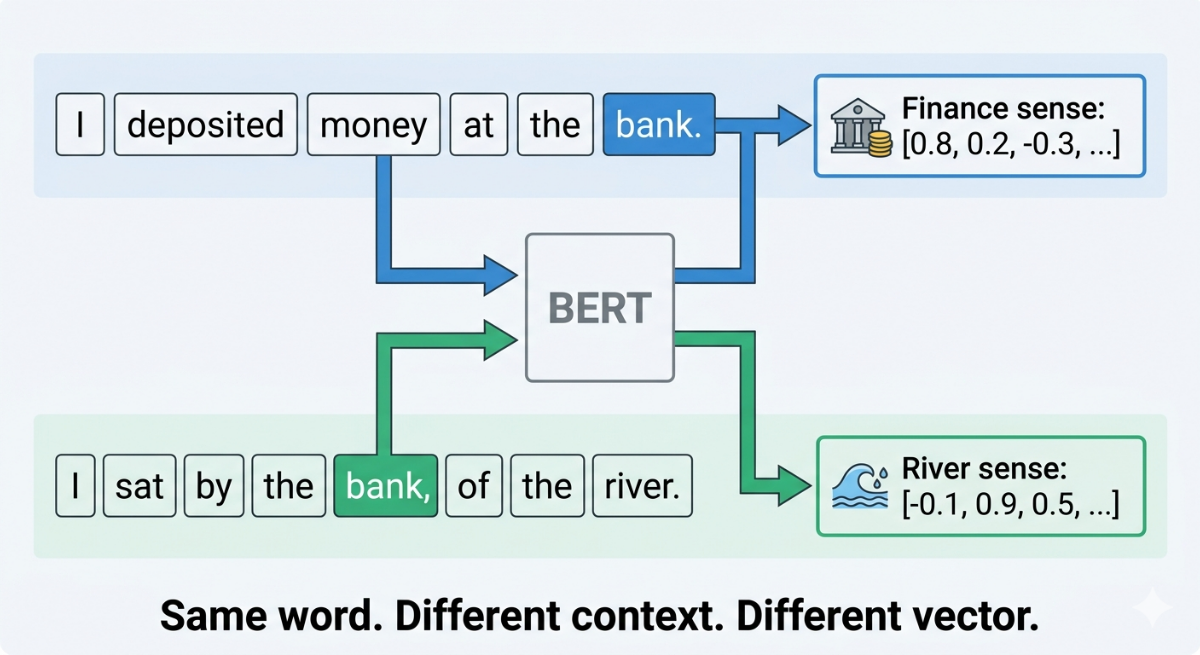
Contextual embeddings give each word a different vector depending on the sentence it appears in. The same word, in a different context, gets a different representation.
This is the core idea behind BERT (Bidirectional Encoder Representations from Transformers), published by Google in 2018.
BERT is a large neural network that reads an entire sentence at once and builds a representation for every word that takes the full surrounding context into account. When it reads "I deposited money at the bank," the word "bank" gets a vector that's been shaped by "deposited" and "money." When it reads "I sat by the bank of the river," the same word "bank" gets a different vector, shaped by "river" and "sat."
The same word. Different sentences. Different vectors. That's contextual embedding.
from transformers import BertTokenizer, BertModel
import torch

tokenizer = BertTokenizer.from_pretrained('bert-base-uncased')
model = BertModel.from_pretrained('bert-base-uncased')

def get_bert_embedding(sentence):
    inputs = tokenizer(sentence, return_tensors='pt')
    with torch.no_grad():
        outputs = model(**inputs)
    # The last hidden state contains one vector per token in the sentence
    return outputs.last_hidden_state

sentence_finance = "I deposited money at the bank."
sentence_river = "I sat by the bank of the river."

embeddings_finance = get_bert_embedding(sentence_finance)
embeddings_river = get_bert_embedding(sentence_river)

# The vector for "bank" will be different in each sentence
print("Finance 'bank' embedding shape:", embeddings_finance.shape)
print("River 'bank' embedding shape:", embeddings_river.shape)
# Both are [1, sequence_length, 768]
# But the numbers at the "bank" position are different between the two
BERT produces a vector with 768 numbers for each word. Those 768 numbers capture the meaning of that specific word in that specific sentence. A completely different 768 numbers would come out for the same word in a different sentence.
This is a much richer representation than anything Word2Vec or GloVe can produce, and it's why BERT-based models dramatically outperformed earlier approaches on almost every language understanding task when it was released.
Sentence Embeddings: Representing Whole Texts
So far we've been talking about embeddings for individual words. But many real applications need a single number representation for an entire sentence or paragraph.
Sentence embeddings are exactly that: a single list of numbers that represents the meaning of a whole piece of text. They're the foundation of semantic search (finding documents by meaning rather than keywords) and RAG systems (where an AI retrieves relevant passages before generating an answer).
The simplest way to get a sentence embedding is to average all the word vectors in the sentence. This works okay for some tasks but loses a lot of information about how the words relate to each other.
A much better approach is Sentence-BERT (SBERT), which is BERT fine-tuned specifically to produce good sentence-level representations. SBERT is trained on pairs of sentences with labels indicating how similar they are. This teaches it to place sentences with similar meanings close together in the vector space.
from sentence_transformers import SentenceTransformer
from sklearn.metrics.pairwise import cosine_similarity
import numpy as np

model = SentenceTransformer('all-MiniLM-L6-v2')

sentences = [
    "Machine learning helps computers learn from data.",
    "Artificial intelligence systems improve through experience.",
    "I enjoy cooking pasta on Sunday evenings.",
    "Deep learning uses neural networks with many layers."
]

embeddings = model.encode(sentences)

similarities = cosine_similarity(embeddings)
print(similarities.round(2))
Output:
[[1.   0.72 0.08 0.63]
 [0.72 1.   0.07 0.54]
 [0.08 0.07 1.   0.06]
 [0.63 0.54 0.06 1.  ]]
Sentences 1 and 2 (machine learning and AI) score 0.72: high similarity. Sentences 1 and 4 (machine learning and deep learning) score 0.63: also meaningfully similar. Sentence 3 (cooking pasta) scores near zero against everything else, which makes perfect sense.
Here's the remarkable part: sentences 1 and 2 share almost no words, yet the model correctly identifies them as highly similar. BM25 or TF-IDF would give them a score of zero because the keywords don't overlap. Sentence embeddings can see past the words to the meaning underneath.
This is what powers modern semantic search, RAG pipelines, and recommendation systems that match content by meaning rather than by exact keyword overlap.
The Full Picture: From Counts to Context
It helps to see all of these techniques side by side to understand where each one fits:
| Method | Type | Understands context? | Captures synonyms? | Use today |
|---|---|---|---|---|
| Bag of Words | Count vector | No | No | Classification baselines |
| TF-IDF | Weighted count vector | No | No | Search, keyword extraction |
| BM25 | Scoring function | No | No | Lexical retrieval, search |
| Word2Vec / GloVe | Fixed word vector | No | Yes | Lightweight semantic tasks |
| BERT embeddings | Context-aware word vector | Yes | Yes | Language understanding tasks |
| Sentence embeddings | Context-aware sentence vector | Yes | Yes | Semantic search, RAG |
Each row in that table solves a problem the previous row had. Count vectors ignore meaning. Static word vectors add meaning but give every word one fixed representation. Contextual vectors make the representation depend on the surrounding sentence. Sentence vectors represent whole pieces of text as a single unit.
You will encounter all of these in real systems, sometimes in the same system. Knowing why each one was created makes it much easier to choose the right one for a given problem.
When to Use Each
Word2Vec or GloVe pretrained vectors are still useful when: - You want a simple semantic representation without the complexity of transformer models - You're working with limited compute or memory - Your task only needs word-level similarity (word clustering, analogies, basic semantic search)
BERT contextual embeddings are the right choice when: - You need to understand word meaning in context (the same word meaning different things in different sentences) - You're fine-tuning a model for a specific task like named entity recognition or question answering - Accuracy matters more than speed
Sentence embeddings (SBERT and similar) are the right choice when: - You need to compare whole sentences or paragraphs by meaning - You're building a semantic search system or a RAG pipeline - You need to cluster documents by topic or find near-duplicate content
What Comes Next
You now understand how text gets represented, from raw counts all the way to rich context-aware vectors. This is the backbone of modern NLP.
The next post puts these representations to work. We'll look at Cosine Similarity: the way NLP systems measure how close two embeddings are, and the engine behind semantic search, document retrieval, and recommendation systems.
Learn This at Fondra Labs
This post is part of our NLP Foundations series, where we build up practical AI knowledge one concept at a time, from text processing basics all the way to the systems powering modern AI.
At Fondra Labs, we teach AI from production reality, not hype. Every topic in this series is here because it genuinely matters when you sit down to build something real.
If this was useful, explore the rest of the blog. We cover machine learning, deep learning, NLP, and the practical skills that turn understanding into building.
Frequently Asked Questions
Javier Aguirre
Teaching AI from production reality, not hype.
Build your AI Foundations
Get the free checklist that production engineers use to avoid these common RAG pitfalls.
Get the Free Guide